Merge Ahead: Don't skip a row

 Anti Join is useful

In this post, we are going to look at how we can use an anti join to figure out which rows of data don't match. This can serve two purposes - it can: 

• Identify data quality errors that we need to fix.
• Provide insight into which records are NOT present in the selected dataset.

Identify data quality errors

Take the two tables below as an example: 

If we choose Left Outer join, the result is: 

We know that the United States is a valid country with an existing population. Same with United Kingdom. So why are we getting null values? 

With this small dataset, it's easy to see that USA and Great Britain/Northern Ireland are the problems - they appear in the Right Table, but they don't exactly match the records in the Left Table.

With larger sets of data, it can be more difficult to find those null values, which equate to mismatches in our data. 

Right Anti Join 

If we choose RIGHT ANTI, the second table will be filtered, to only give results that do NOT appear in the first table. In this case, I want view rows that appear in the Population table but do not appear in the Sales table, so that I can identify why United States and United Kingdom have both returned null for population: 

When doing a RIGHT ANTI join, we end up with many columns of unhelpful null values, but when we expand the Merge column, we get the results we are looking for. Below you can see the countries that have no matching record in the Sales table, and we can easily identify which should match United States and United Kingdom: 

Now that we know the problem, we can fix the data. 

Transform Data to Improve Data Quality

In this example, we only need to do two simple fixes in our Population table: 

• Replace USA with United States
• Group all countries in United Kingdom

Both of these fixes can be done directly in Power Query. 

Replace Values

United States can be fixed with a simple Transform > Replace Values.

Group by

United Kindgom needs two steps. 

First, we will replace the values to find: 

• Northern Ireland
• Great Britain

And replace all with "United Kingdom".

Then, we will Group By Country. 

NOTE: Group By is a great way to ensure the column(s) selected in your Group By have unique values. This is highlighted extensively in my other Merge Ahead post and will ensure I do not get any unwanted duplicate data in my merge!

My Right Anti join is now an EMPTY table. 

And my Left Outer join now looks like this: 

Provide Insight into which records are NOT in selected data

For this example, I am going to use Olympic Medal data which is readily available from Wikipedia. For stable data matching this post, you can use: 

• Medals by Country
• Population by Country

Objective: 

Our goal is to see which countries have never won any Olympic medals.

Select Table 4 from the Population by Country website. Rename the query to 'Population'.

Select Unranked medal table (sortable) from the Population by Country website. Rename the query to 'Medals'.

Transform Medals table

Rename the first column to 'Country'

Extract text before delimiter (

Trim Country column

Transform Population table

Rename the first column to 'Country'

Extract text before delimiter (

Extract text before delimiter [

Trim Country column

Left Anti Join

If we choose Left Anti Join, we will need Population as the Left table and Medals as the Right table in order to see which countries exist in the Population table but have no record of winning any Olympic medals in the Medals table.

Note a Left Anti Join does not require us to keep the null columns. We will get a column of Table values, but because we have chosen an Anti join, all Tables in this column will be empty, so we can remove this column. 

Result:

Now we can see which countries have not won any Olympic medals: 

Some of these results, like the United Kingdom, we will recognize and are related to Data Quality Errors. Many of these results though provide insight into opportunity for growth.

Conclusion

An anti join can help add insight to your reporting as well as provide you with the information you need to cleanse and transform your data effectively. Use a Left Anti join with the "Merge Queries as New" option and remove that unneeded column of empty Table values you get and simply focus on the filtered rows that result from the unmatched data. 

Merge Ahead: One for one

 Proper Merging Technique

Merging tables in Power Query is as challenging as it is to merge on the road, and it's just as important to get it right. If you make a mistake when merging tables, you could end up with corrupted data! In this post, we will look at why merging can cause unwanted duplication in your data and how to avoid this.

When driving, we are often told to 'Merge like a zip' - meaning for every car in the left lane, only one car from the right lane is allowed. If we replace the word 'car' with 'row' and 'lane' with 'table', we can apply this same technique to Power Query: 

For every row in the left table, only one row from the right table is allowed. 

While this is not always the case, it is a good technique to follow if you don't want to duplicate the data in your left table. On the road we can't copy the cars in the left lane, but in Power Query that's exactly what happens with our data - it gets copied. This duplication of data can throw off your report and cause a bigger headache than a fender bender.

Definition: Merge

A merge starts with a long data table and pulls in data from related lookup tables to create one flattened data table. You may be familiar with the VLOOKUP, HLOOKUP, INDEX or MATCH functions in Excel, merging tables can achieve the same result, but much faster and has the capability to pull in multiple fields at once.

Join Kind

A merge can also be used to filter out unwanted data (such as invoices that have already been processed or products which have not been sold). This is achieved by selecting the correct Join Kind for the merge.

Power BI offer six options for Join Type when merging tables.

Left Outer – All data from the first table, matching data from second

This is the typical result achieved through VLOOKUP in Excel. In the example of a Sales table of all sales for the month merged with a Product table containing a list of all product information, this would be a great way to pull in product name, price and cost based on the product ID in the Sales table. If a product wasn’t sold that month, it will not be pulled through into the merge. However, if there was a sale for a product not in the product list, this sale will still be pulled through into the merge, just with empty fields for product name, price, etc.

Right Outer – All data from second table, matching data from first

This is similar to the Left Outer join, but when your tables are in reverse order.

Full Outer – All rows from both

This is useful if you want to see empty data. In the Sales and Product table’s example above, this would also pull through the product information for snow boots and shovels, even if there were no sales for them in February. The columns for sales date, etc. would be empty.

Inner – Only matching rows

This is a great way to filter your data while merging with additional columns. Continuing the example from above, this could be useful for someone from the clothing department. They start with the Sales table of all sales of all products for the entire company. Then they merge with a Clothing Products table which only has the products from their department. An Inner join will result in a table with sales and product info for clothing products only if they were sold that month.

Left Anti – Rows only in first table

This is a great way to filter your data. Because it pulls through rows only in the first table, you won’t get any additional columns. In the example above we could merge the Sales table with a list of products available on the website. The Left Anti join will leave us with only the sales for products that are not available online, thereby showing us the most popular products that we might want to make available on the website.

Right Anti – Rows only in second table

This achieves similar results to the Left Anti join but with the tables in reverse order.

Improper Technique: Merge adds rows

For merge tables with a Left Outer join, the second/right table should have unique values in the column(s) you select as the matching columns. 

For example: 

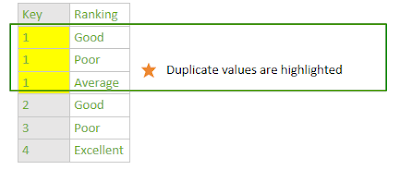
Consider the below two tables, merging them as a Left Outer Join, using the Key columns as the matching columns.

Merging with: 

Desired Result:

(No added rows)

Ideally, we want to have the same number of rows that we started with - one for each country. However, what do we put for USA ranking? 

There are duplicates in the Key column in the second table, so when we do a Merge, Power BI or Excel won't know which row to choose for Key 1. 

Options without adding rows are: 

2 (count of rankings)

Good (first ranking)

Average (last ranking)

These are all AGGREGATIONS of our data, and I do NOT recommend doing an aggregate merge as it can decrease the overall performance of your query.

So, if we do an expanded Left Outer Merge, what will our actual result be?

Actual Result:

(Added rows)

In the image below, you can see that when we expand the Ranking column from our second table, this adds two extra rows to our data!

 The impact of this on your report can be as catastrophic as failing to merge like a zip on the road.

Proper Technique: Use Unique Key

To achieve the desired result, we must use a UNIQUE KEY column as the matching column for our Table 2 merge. You can use the Column distribution in Power Query to see if the first 1000 rows of your column has unique values, and the Column profile to easily identify which values are NOT unique: 

Ideally, you would have a unique key in your data set. This might mean you need to combine two (or more) columns, such as: 

• Country, Region
• Order Number, Order Line
• Date, Time

If you don't have a unique key in your dataset, consider WHY you are doing this merge and WHAT information you wish to report on. In some cases, you may want the duplicate rows (note this is very uncommon).  

In this example, I only care to display the latest ranking, so I need to ensure my data is sorted, and then remove the duplicates only on the column (or columns) which will be used in the matching for the merge. Note there are no exact duplicates when we look at the entire table - each ranking for Key 1 is different. 

We need to focus only on the Key column to remove the duplicates. Let's assume this data has come in date order, so no need to sort. So, we can remove all duplicate Key values, leaving us only with the first row of each Key: 

To remove duplicates: 

1. Select the column or columns that will be used as the matching column(s) in the Merge. 
2. With the columns selected, in the Home tab > Remove Rows > Remove Duplicates. 
3. Note the formula bar - this operation only looks at the SELECTED COLUMNS, in this case "Key", to decide which duplicates to remove, and keeps the top row only.

NOTE: You MUST select the key columns first. If you remove duplicates on the entire table, you are NOT guaranteed unique values in the key columns. If you select only the key columns and then remove duplicates, you are GUARANTEED unique values in the key columns combined.

Now, we can perform our merge. 

And expand the Ranking column: 

Our final result still has only 4 rows: 

Conclusion

When doing a Merge in Power Query, we must use a Unique Key if we do NOT want to duplicate records of our data. To keep things simple, that unique key must typically be in the second/right table of the Merge for any join kind.

DateKey: How to relate your date data

If the idea of relationships in Power BI is completely new to you, you may wish to review some of my previous posts, such as Part II: It's Complicated Relationships in Power BI.

To give a quick recap, in order to create successful relationships between two tables, we should always check a few things: 

• Does the data type match? 
• Are they in the same format? 
• Is there a one to one or one to many cardinality? 

In this post, we will look more closely at what we mean by 'same format' and use the most common example of where we get this wrong - dates. 

Assuming both your date table and fact table use Date/Time data type, you may find your data is in the following format: 

FACT Table

DimDate Table

Although both sets of data are in the format M/D/YYYY hh:mm:ss AM/PM, what difference do you notice? 

Look more closely at the DimDate table times - each row has 12:00:00 AM for the time. This is true of any TRUE date table - we are only allowed a single row per date, so we must have only ONE time for each date. Usually that time is 12:00:00 AM. 

How often does your data have exactly 12:00:00 AM as its time? In this example, how often is the submit date at exactly 12:00:00 AM? Almost never. 

So if we look at our rules again, let's see where the problem lies: 

• Does the data type match?  Yes - both are Date/Time.

• Are they in the same format?  Yes - both are M/D/YYYY hh:mm:ss AM/PM

• Is there a one to one or one to many cardinality? Yes - DimDate has unique values for Date.

So what's the problem? Our M/D/YYYY hh:mm:ss AM/PM format does not allow for any matching data. So we really need to add another rule to our list: 

• Is there a matching record in the Dim table for every record in the Fact table?

In this rule we fail. 4/22/2019 4:58:56 PM will NEVER appear in the DimDate table - it only shows 12:00:00 AM. So, we need to create a DateKey column that will follow all of our three initial rules AND provide matching records for each row of data. 

Creating DateKey

I like to use YYYYMMDD for my DateKey, and I add a new column in Power Query for every date that will need to be used in a relationship in Power BI.

Open Power Query Editor. Click the Add Column tab > Custom Column. 

If your data has DateTime column that you want to get DateKey of, use this formula: 

=DateTime.ToText([Date], "yyyyMMdd")

If your data has Date column that you want to get DateKey of, use this formula: 

=Date.ToText([Date], "yyyyMMdd")

Click OK to create your column. 

Repeat for ALL Date fields in your data that will be used in relationships.

Close & Apply or Close & Load your changes. 

Now you should be able to create relationships in Power BI or Excel with greater success.